MinCell 1 with quotas
The code for this example is available in our main GitHub repository. https://github.com/TP-Watson/py_cFBA
We start with a simple toy model of a minimal cell. This is the same example that is presented in our article [1]. A schematic of the model with its corresponding S matrix can be seen in the following scheme:

In this tutorial we will continue with the simulations from MinCell 1, in which the growth of the system was optimized (reaching a max growth of 1.8). However, in this example we will implement quota components.
Simulation with different quotas
As explained in Method Constraints, in cFBA you can define quotas which are specific constraints to each imbalanced metabolite at a speific time point. These quotas can be classified as:
Maximum quota: inequality constraint for which an imbalanced metabolite exceed.
max.Minimum quota: inequality constraint for which an imbalanced metabolite must be at least.
min.Equality quota: exact constraint for the concentration of an imbalanced metabolite.
equality.
In the previous example we did not define quotas, so the variable quotas was an empty list. In this example, we will define several different quotas for imbalanced metabolites. The definition of these quotas is done as follows:
# Quotas for the model
quotas = [
#   ['type',     'metabolite', time, value]
    ['equality', 'Storage',    0,    0.5],
    ['max',      'Biomass',    2,    1],
    ['equality', 'Enzymes',    0,    0.5]
]
These definitions indicate that:
At time point 0, Storage should be exactly 0.5 mol/gDW.
At time point 2, Biomass should be at least 1 mol/gDW.
At time point 0, Enzymes should be at least 0.5 mol/gDW.
We then perform the optimization as done in the preious example.
# Find the optimal alpha value
print('Time simulation:')
alpha, prob = find_alpha(cons, Mk, imbalanced_mets)
print('Growth of the system: {:.2f}'.format(alpha))  # Print the optimal alpha value

# Retrieve the solution: fluxes, amounts, and time points
fluxes, amounts, t = get_fluxes_amounts(sbml_file, prob, dt)
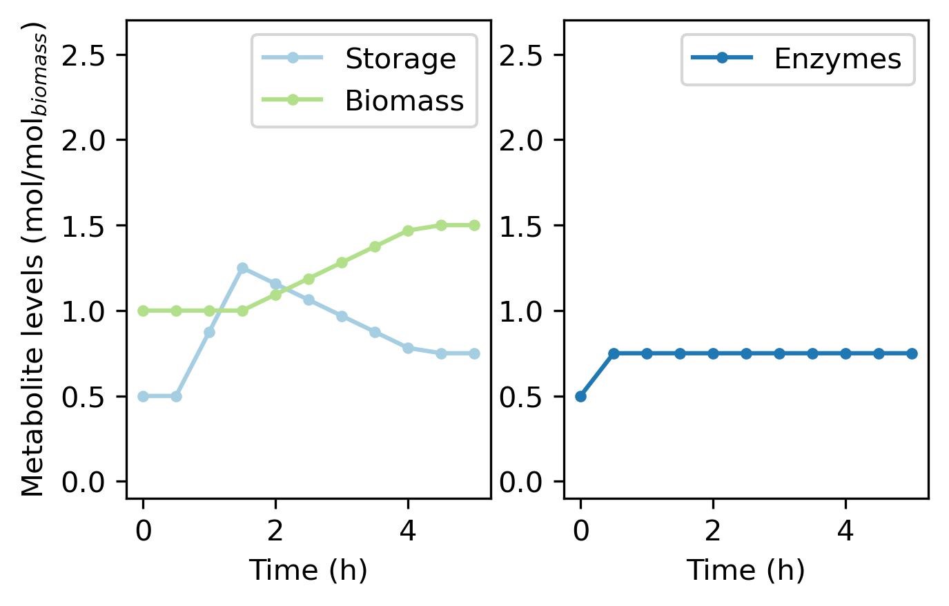
The resulting growth of the system is lowered, since we forced the model to start with higher storage concentrations. In the first example, the optimal solution was that in which storage started with a concentration of 0 mol/gDW at the begining.
Time simulation:
0.02 min
Growth of the system: 1.50
Now we can plot the profiles of the metabolites.
# Plot the metabolite changes over time
colors = ['#a6cee3', '#1f78b4', '#b2df8a']  # Colors for plotting

plt.figure(figsize=[5, 3])
plt.subplot(1, 2, 1)
plot_met('Storage', colors[0])  # Plot 'Storage' metabolite levels
plot_met('Biomass', colors[2])  # Plot 'Biomass' metabolite levels
plt.ylim([-0.1, 2.7])  # Set y-axis limits

plt.subplot(1, 2, 2)
plot_met('Enzymes', colors[1])  # Plot 'Enzymes' metabolite levels
plt.ylim([-0.1, 2.7])  # Set y-axis limits
plt.ylabel(None)  # Remove y-axis label


plt.savefig('MinCell_01_3.jpeg', bbox_inches = 'tight', dpi = 300)
plt.show()  # Show the plots
And the corresponding fluxes.
# Plot the flux changes over time
colors = ['#e41a1c', '#377eb8', '#4daf4a', '#984ea3']  # Colors for plotting

plt.figure(figsize=[5, 3])
plot_flux('vstorage', colors[0])  # Plot 'vstorage' flux
plot_flux('venzymes', colors[1])  # Plot 'venzymes' flux
plot_flux('vgrowth', colors[2])  # Plot 'vgrowth' flux
plot_flux('vupt', colors[3])  # Plot 'vupt' flux


plt.savefig('MinCell_01_4.jpeg', bbox_inches = 'tight', dpi = 300)
plt.show()  # Show the plots

With this, you have finalized the tutorial on MinCell 1. You can move onto the next examples in which: